TRANSIENT ANALYSIS
CIRCUIT

One of the most complex and intriguing capabilities of the SPICE algorithm is the Transient Analysis. How do we take a collection of resistive and energy-storage components, then find its time response to an arbitrary input waveform? Yes, you could formulate and solve the differential equations to get the response versus time, but SPICE is not a differential equation solver. However, like non-linear circuit analysis, by first transforming the energy-storage components into their linear companion models, you can use the Nodal Analysis to find your answer.
NUMERIC INTEGRATION
Back in school, we learned how to formulate differential equations to describe, say, an RC circuit. Then, given some input, we applied our calculus techniques to find a nice analytical function for the output. But SPICE has no such analytical abilities. Instead, it attempts to find an approximation to the analytical solution at discrete time points using numeric integration. If you plotted the all the discrete points, it should match the graph of analytical function.
Let's see how numeric integration works. Knowing a function at some point in time tn, how could you approximate the function at a future time point tn+1? Here's one approach. What if you looked to the slope of the curve to tell you, at least locally, where the voltage is going? Then, simply multiply the slope by the time step h = Δt = tn+1 - tn and add it to the present voltage - that should get you in the neighborhood at least. You can write the approximation as
![]()
Graphically, it looks something like this.

Numeric integration applied to approximate the next voltage.
This is known the forward-Euler (FE) integration formula. Is the approximation perfect? Unfortunately no. As you can see, there's some error between the actual curve and your estimated point xn+1. Can you make it better? Yes, either reduce the time step or improve on the formula.
The FE formula is so intuitive, but its not the best method. Another method, the backward-Euler (BE), uses the slope at x n+1, rather than the one at x n, to predict the next voltage.
![]()

Backward-Euler formula applied to predict the next voltage.
SPICE actually uses the BE formula (along with several others discussed below.) This method is more accurate and less sensitive to size of the time step compared to the FE method.
CAPACITOR COMPANION MODEL
Okay, we're approaching our overall goal of transforming an energy-storage component into its equivalent linear components. For example, a capacitor is transformed using a two step process:
Step 1. Apply numeric integration to the current-versus-voltage relationship of
a capacitor.
Step 2. Use the result to develop a linear companion model well-suited for
Nodal Analysis to calculate the circuit's output waveform.
First step, write the equations that tell the story of a capacitor's voltage-current-charge relationships.
V = Q / C
I = dQ / dt
Next, apply the BE formula to predict the capacitor's voltage at the next time point.
![]()
Let's try to get this equation in terms of voltage and current only without any derivatives. Swapping V = Q / C in the second term, you get
![]()
Finally, substituting I = dQ / dt, you get an equation in terms of voltages and currents only!
![]()
So, how do we create a linear companion model? Just rearrange it such that the current is in terms of the voltages.
![]()
You can think of (C / h) as a conductance Geq, because multiplying it by V produces a current.
![]()
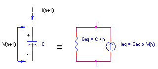
Now, we implement this equation with simple circuit components.

Linear companion model of a capacitor using the BE formula.
Conductance Geq describes the part of C1’s current dependent on its new voltage Vn+1; current source Ieq describes the other part based on the past voltage Vn.
NODAL ANALYSIS
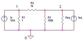
We treat the capacitor model like any other linear components in the circuit

and develop the nodal equations.

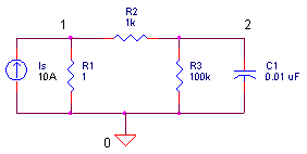
To solve for V1 and V2, let's first simplify bookkeeping by letting G11 = 1/R1 + 1/R2, G12 = -1/R2, G21 = -1/R2, G22 = 1/R2 + 1/R3 + Geq, I1 = Is and I2 = Geq∙V t. The equations become
![]()
Solving the two equations, we get

![]()
We'll use these next in our Excel spreadsheet.
TRANSIENT ANALYSIS
Let's fire up the transient analysis machine and see how she flies. Download and open the spreadsheet TRANSIENT _SIMULATION.XLS. Under the variables shaded in light blue, enter R1, R2, R3, C1 and h.
|
R1 |
R2 |
R3 |
C1 |
h or ΔT |
|
1 |
1000 |
100000 |
1E-5 |
5E-4 |
What kind of waveform do you expect at node 1? Current source Is and R1 create a voltage V1 = Is ∙ R1 = 1 A ∙ 1 Ω = 10V. (There's little effect of R2 and C1 on the impedance of R1.) Components R2 and C1 form a low-pass filter. (Since R3 = 100 kΩ is so large, it's basically out of the picture.) And, we know that a low-pass RC filter responds to a step input with an exponential curve at its output. With a time constant of R2 ∙ C1 = 1 kΩ ∙ 10 μF = 10 ms, the waveform should rise to about 63% in 10 ms.
The spreadsheet calculates the conductance matrix G according to the equations
| G11 | G21 | G12 | G22 |
| 1/R1 + 1/R2 | -1/R2 | -1/R2 | 1/R2 + 1/R3 + Geq |
Finally, the current vector is formed
| I1 | I2 |
| Is | Geq∙V2' |
where V2' is the voltage across the capacitor from the previous row. All that's left is to solve the equations for V1 and V2 using the equations found in the Nodal Analysis section above.
Check out the graph of V2 - an exponential curve as expected! ( Fascinating, how a non-linear curve is generated by a collection of linear components!) Play with the R2 and C1 values. What happens to the rise time? Try values like R2 = R3 = 1k. What voltage does the output settle to?
SPICE INSIGHT Return the component values to R1 = 1 Ω, R2 = 1 kΩ, R3 = 100 kΩ and C1 = 10 μF. Does the output rise to about 63% in 10ms? Increase the time step h, from 0.5ms to 2ms. What happened? The output overshoots 63% in 10 ms. No wonder, the time constant and time step size have a similar magnitude. Most likely the BE formula and the relatively large time step size introduced some errors. In the actual SPICE algorithm, the time step is adjusted dynamically during the simulation to minimize the error.
In the spreadsheet, the Is column defines the signal source - a current pulse created by values of 10 A followed by values of 0 A. As an alternative waveform, try defining a sinewave using the Excel SIN function in column (F) using the time values in column (M). The cell formula might look like SIN(100*M9). What should the output look like? Depending on the frequency, you could see a sinewave that's been attenuated and possibly shifted in time.
OTHER NUMERIC INTEGRATION FORMULAS
Besides the Backward Euler formula, other effective methods have emerged. For example, the Trapezoidal formula calculates the average slope of the present and next time point to approximate the next solution.
![]()
where
![]()
to simplify notation a bit. This new formula also means we have to throw out our previous linear companion model for the capacitor and construct a new one.
The Gear-2 formulation predicts the next point using information from the present and two from the past!
![]()
Gear-3 uses three solutions from the past and so on.
Why so many different formulas? Each one has its own strengths and weaknesses. What makes them strong or weak? There's two main characteristics.
Accuracy - how much error (Local Truncation Error) each method introduces.
Stability - Does the error accumulate (that's bad) or decrease to zero (that's good!)
over time?
Depending on the expected waveform, one method may have an advantage over another. Here's a quick summary of the available integration methods.
| (FE) Forward Euler | Not very accurate, not used by SPICE. | ||
| Trapezoidal | Better accuracy than stability, may oscillate in some cases. Default in some SPICE versions. | ||
| (BE) Backward Euler | Average accuracy and stability. Default in some SPICE versions. | ||
| Gear-2 | Better stability than accuracy. Most stable method. |
OTHER LINEAR COMPANION MODELS
Okay, a companion model for a capacitor has been created above, but what about other components - inductors and the charge-storage mechanism in diodes, BJTs, JFETs and MOSFETs? For each of these SPICE must create a linear companion model based on the device's defining equations and the type of numeric integration. Not only have the defining equations changed over the years, but many SPICE versions dynamically change the numeric integration method during a simulation for optimal results. A huge task, no doubt, and one that SPICE companies work continuously to improve upon.
NEED MORE INFO?
Here are some gold mines of information about the SPICE engine.
SPICE2: A Program to Simulate Semiconductor Circuits, Lawrence W. Nagel, Memo UCB/ERL M520, 1975, University of California, Berkeley, CA.
The Spice Book, Andrei Vladimirescu, John Wiley & Sons, Inc., 1994,
ISBN 0-471-60926-9.Inside SPICE, Ron Keilkowski, McGraw Hill, 1994, ISBN 0-07-913712-1.
For more info on these and other books go to the Bookshop.
About SPICE |
SPICE Basics | Running SPICE
| CIRCUIT COLLECTION |
SPICE Commands
SPICE Demos and Downloads | About Us | Contact Us | Home |
Search
© 2003 eCircuit Center