NODAL ANALYSIS
After simulating circuits for some time, I began to ask myself - how does this SPICE program actually work? What mathematical tricks does the code execute to simulate simple to complex electrical circuits?
After some searching and digging, some answers were uncovered. At the core of the SPICE engine is a basic technique called Nodal Analysis. It calculates the voltage at any node given all resistances (conductances) and current sources of the circuit. Whether the program is performing DC, AC, or Transient Analysis, SPICE ultimately casts its components (linear, non-linear and energy-storage elements) into a form where the innermost calculation is Nodal Analysis.
WHAT IS NODAL ANALYSIS?
Kirchoff discovered this: all of the currents entering and leaving a node sum to zero! And, these currents can be described by an equation of voltages and conductances. If you have more than one node, then you get more than one equation describing the same system (simultaneous equations). The trick now is finding the voltage at each node that satisfies all of the equations simultaneously.
Circuit Example Here’s a simple circuit example.
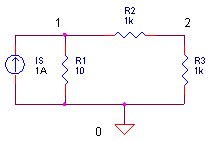
We'll choose the following convention: the currents leaving the node are considered positive. This (and Ohm's law) enables you to write two equations for the two nodes as

Because our mission is to calculate the node voltages, let’s reorganize the equations in terms of V1 and V2.

So here sit V1 and V2 in the middle of two different equations. The trick is finding the values of V1 and V2 that satisfy both equations. But how?
SOLUTION #1 – WORK THE EQUATIONS
Just roll up your sleeves and solve for V1 and V2. Before we begin we’ll make bookkeeping easy by writing the resistors in terms of total conductance: G11 = 1/R1 + 1/R2, G12 = -1/R2, G21 = -1/R2 and G22 = 1/R2+1/R3. The system equations now look like this.
![]()
First, solve the second equation for V1
![]()
Then, stick this into the first equation and solve for V2

Okay, it’s a little messy, but we’ve got V2 described by circuit conductances and Is only! After V2 is calculated numerically, stick it back into V1 = – G22 ∙V2 / G21 and there you have it, circuit voltages V1 and V2 that satisfy both system equations.
SOLUTION #2 – THE MATRIX
Solution #1 looks reasonable for simple circuits, but what about medium or large circuits? The bookkeeping of terms spins out of control quickly. What’s needed is a more methodical and efficient solution: Enter the Matrix. Here’s the set of nodal equations written in matrix form.

Or, in terms of total conductances and source currents

Treating each matrix as a variable, you can write
G ∙ v = i
In the matrix world, you can solve for a variable (almost) like any other algebraic equation. Solving for v you get
v = G-1∙ i
Where G-1 is the matrix inverse of G. ( 1 / G does not exist in the matrix world.) This equation is the central mechanism of the SPICE algorithm. Regardless of the analysis – AC, DC, or Transient – all components or their effects are cast into the conductance matrix G and the node voltages are calculated by v = G-1∙ i , or some equivalent method.
LINEAR DC ANALYSIS
Armed with Nodal Analysis and an Excel spreadsheet, you can perform Linear DC Analysis on the circuit above. Download and open the spreadsheet LINEAR_DC_ANALYSIS.XLS. Enter the circuit values under the variables shaded light blue.
|
R1 |
R2 |
R3 |
Is |
|
10 |
1000 |
1000 |
1 |
How much voltage would you estimate at nodes 1 and 2?
You can expect V1 = Is ∙ R1 =
1 A ∙ 10 ohms = 10V. That’s because R2
and R3 have little effect on 10 ohms. At node 2, the simple R2-R3 divider
should produce about V2 = 5V.
First, the spread sheet calculates the conductance matrix G
|
0.101 |
-0.001 |
|
-0.001 |
0.002 |
according to the equations
|
1/R1 + 1/R2 |
-1/R2 |
|
-1/R2 |
1/R2 + 1/R3 |
Next, Excel inverts G and multiplies the result G-1 by i to get v. ( See how Excels inverts and multiplies matrices below.)
G-1 x i = v
|
9.95 |
4.98 |
x |
1 |
= |
9.9502 |
|
4.98 |
502.49 |
|
0 |
|
4.9751 |
And there you have it, just like the SPICE engine, we’ve computed the circuit’s voltages! Pick other values for R1 like 1 or 100 Ω. Does the output scale up and down as expected? Change R2 or R3. Vary Is or change its polarity.
HANDS-ON DESIGN Try adding another resistor to the circuit. For example, place R4 in parallel with R3. Write out the nodal equations. Then include R3 in the cell formulas that form G. The Excel formulas should effectively calculate the following.
|
1/R1 + 1/R2 |
-1/R2 |
|
-1/R2 |
1/R2 + 1/R3 + 1/R4 |
THE SPICE CIRCUIT
To verify the results our nodal analysis, you can run a simulation of DC_LINEAR_CKT.CIR. Download the file or copy this netlist into a text file with the *.cir extension.
LINEAR_DC_CKT.CIR - SIMPLE CIRCUIT FOR NODAL ANALYSIS
*
IS	0	1	DC	1A
*
R1	1	0	10
R2	1	2	1K
R3	2	0	1K
*
* ANALYSIS
.TRAN 	1MS  10MS
* VIEW RESULTS
.PROBE
.END
Although it runs a Transient Analysis, it essentially computes a DC Linear Analysis because no non-linear elements or charge-storage devices exist in the circuit. Plot V(1) and V(2). Utilize the cursor, if needed, to get an accurate measurement. Do the voltages from SPICE and Excel agree?
EXCEL MATRIX OPERATIONS
Excel provides handy matrix functions for getting our hands on the nodal analysis example. Matrix functions are entered like any other Excel function except for one trick. Instead of pressing ENTER after entering a function, you need to hit CTRL-SHIFT-ENTER simultaneously!
► MATRIX INVERSION
Here are the steps to calculate the matrix inverse of G in the file LINEAR_DC_ANALYSIS.xls.
1. Select the range of cells (B16:C17) to hold the inverse result.
2. Type the formula MINVERSE(B10:C11) where B10:C11
defines the matrix to be inverted.
3. Press CTRL-SHIFT-ENTER.
► MATRIX MULTIPLICATION
Multiplying two matrices is just as easy.
1. Select the cells (G16:G17) to hold the multiplication result.
2. Type the formula MMULT(B16:C17, E16:E17) where B16:C17
represents the square matrix and E16:E17 represents column
matrix to be multiplied.
3. Press CTRL-SHIFT-ENTER.
THE MATRIX SOLUTION - GOOD NEWS, BAD NEWS
The good news is that the matrix form of system equations can be easily expanded to larger circuits. The bad news lies in finding v. There are several paths to answer. Why so many? Some are more efficient then others. Briefly, here are three techniques to solve the matrix equation for v.
1. MATRIX INVERSION
Although a very straight forward formula exists (Cramer’s Rule) to calculate the inverse of G, it’s very inefficient for large matrices.
2. GAUSSIAN ELIMINATION
Matrix equations posses an amazing character trait! You can scale, add, or subtract rows of G and i without disturbing the solution to v. By cleverly choosing these operations, you can transform G into an Upper Triangular matrix, where all of the elements below the diagonal are zero! This makes finding v a snap using a technique called Backward Substitution. This method requires much less computational effort than Matrix Inversion.
3. LU FACTORIZATION
For maximum efficiency, SPICE actually uses an extension of Gaussian Elimination. The conductance matrix G is first factored into two matrices G = L U where L (Lower Triangular) stores the scale factors of Gaussian Elimination and U (Upper Triangular) stores the result of Gaussian Elimination. Then, the equation is solved for the node voltages
v = U-1 L-1 i
The inverses of L and U may not actually calculated. Instead, the equivalent is achieved by Forward and Backward Substitution steps. The advantage over Gaussian Elimination is that v can be solved repeatedly for different current sources i by only performing the forward and backward substitution steps. This comes in handy when SPICE performs different analysis like sensitivity, noise and distortion for the same circuit!
WHAT ABOUT VOLTAGE SOURCES?
You may have noticed that nodal analysis does not accommodate a voltage source. What can be done? In the early days, voltage sources were defined with a small series resistor, representing the internal resistance of the source. Then, the V with series R was converted into its Norton Equivalent of I with parallel R. This alternate current source fit nicely into the Nodal System and all was right with the world.
Later, a clever method was hatched to include voltage-defined components called Modified Nodal Analysis (MNA). In this system, much of the equations looked just like Nodal Analysis with rows of equations added describing the influence of the voltage sources.
WANT MORE INFO?
Here are some great sources of information on simulation.
SPICE2: A Program to Simulate Semiconductor Circuits, Lawrence W. Nagel, Memo UCB/ERL M520, 1975, University of California, Berkeley, CA.
The Spice Book, Andrei Vladimirescu, John Wiley & Sons, Inc., 1994,
ISBN 0-471-60926-9.Linear Algebra and Its Applications, Gilbert Strang, Academic Press, 1980,
ISBN 0-12-673660-X.
© 2003 - 2024 eCircuit Center