Non-Linear DC Analysis

eCircuit Center

SPICE Topics

NON-LINEAR DC ANALYSIS

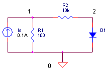
CIRCUIT

Using Nodal Analysis, you can find the voltage at every node in a DC linear circuit. But the technique runs into a brick wall if any non-linear components, such as a diode, appear in the circuit. Turns out, the solution is still within reach. The secret lies in first transforming the non-linear components into something usable by Nodal Analysis. The technique requires a little guessing, and a lot more trips to the nodal equation solver than is needed by a linear circuit.

DIODE MODEL

As an example, let's look at a very non-linear component, a diode. Its current versus voltage relationship is described by

where IS is the saturation current and Vt the thermal voltage.

Using a little tunnel vision around an operating voltage Vdo, you can approximate the behavior by a line tangent to its ideal curve.

Diode characteristic curve and tangent line.

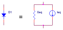
How does the tangent line help circuit analysis? A straight line can be modeled using linear components - a parallel combination of a conductance Geq and a current source Ieq! The conductance Geq is simply the slope of the tangent at the operating point Vdo.

The term Ieq is the point where the tangent slices through the y-axis.

Here's the non-linear diode transformed into its linear companion model.

NODAL ANALYSIS

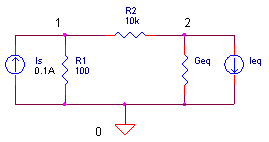
Now, we can treat the diode like any other linear component in the circuit

and develop the nodal equations. (See Nodal Analysis for quick review.)

We can easily solve for V1 and V2. First, to simplify bookkeeping, let G11 = 1/R1 + 1/R2, G12 = -1/R2, G21 = -1/R2, G22 = 1/R2+Geq, I1 = Is and I2 = - Ieq. The equations reduce to

Then work the equations directly to get

Finally, stick the calculated V2 value into the next equation to get V1.

(We'll use these later in our Excel spreadsheet.)

REPEAT NODAL ANALYSIS AS NEEDED
(NEWTON'S METHOD)

Remember, the diode's linear companion model was created at some operating point. But, which operating point? Well, initially we don't know - we can only guess at a trial operating point. After solving the Nodal equations, the voltage found across the diode serves as the next trial operating point and a new companion model is created. Again, the nodal equations are solved and the next trial operating point is found. Repeat as necessary until it converges to a solution.

How do you know when you've reached a solution? If the changes in circuit voltages and currents, between one iteration (n) and the last iteration (n-1), are smaller than some limit, then you've arrived at a solution. The whole thing looks like this:

Step 1. Guess at the diode's initial trial operating point.

Step 2. Create linear companion models.

Step 3. Solve Nodal Equations.

Step 4. Convergence?

            | V(n) - V(n-1) | < VLIMIT and | I(n) - I(n-1)| < ILIMIT ?

            No - Use the calculated diode voltage as new trial operating point
                    for another iteration. Start again at Step 2.

            Yes - Jump to Step 6.

Step 6. Stop iterations, solution reached!

And there in a nutshell is Newton's method (or the tangent method) of solving non-linear equations

Top↑

NON-LINEAR DC ANALYSIS

Let's jump in the non-linear waters with an Excel spreadsheet for our diode circuit. Download and open the spreadsheet NON-LINEAR_DC_ANALYSIS.XLS. Under the variables shaded in light blue, enter the diode's reverse current IS and thermal voltage Vt at 27 °C. Next, enter the resistors R1, R2 and current source Is.

IS	Vt	R1	R2	Is
1E-15	0.025875	100	10000	0.1

How much voltage would you estimate at node 1? You can expect V1 = Is ∙ R1 =
0.1 A ∙ 100 Ω = 10V. That’s because R2 = 10 kΩ and the diode will have little effect on R1's 100 Ω.

Now, it's time to enter your guess at a trial operating point for the diode, say 0.9V. From this guess, Excel calculates the diode current Id and its companion model values Geq and Ieq (see equations above).

Vd	Id	Geq	Ieq
0.9	1.28	4.93E+01	-4.31E+01

Just to the right, the spreadsheet calculates the conductance matrix G according to the equations

G11	G21	G12	G22
1/R1 + 1/R2	-1/R2	-1/R2	1/R2 + Geq

Finally, the current vector is formed

I1	I2
Is	-Ieq

Okay, here comes the main objective - solve the equations for V1 and V2. The voltages are calculated using the equations found in the Nodal Analysis section above.

V1	V2
9.91	0.8741

Notice the next row. The diode voltage V2 from the previous row is placed in column B as the new trial operating voltage! Another round of calculations then begins.

How do you know if V1 and V2 are correct? Just look at the change in the diode voltages and currents during the last iteration. The last 2 columns holds these values. As you can see, by the 8th iteration the change is small and getting smaller. You can say, the solution is converging!

ALGORITHM INSIGHT The number of iterations it takes depends a lot on your initial guess at the diode voltage. Try another initial guess like 0.65 or 0.95V. How many iterations did it take? Try changing Is, R1 and R2. What effect does it have on the voltages and number of iterations?

Top↑

THE SPICE CIRCUIT

To verify our results, you can run a simulation of NON-LINEAR_DC_ CKT.CIR. Download the file or copy this netlist into a text file with the *.cir extension.

NON-LINEAR_DC_CKT.CIR - SIMPLE NON-LINEAR CIRCUIT
*
IS	0	1	DC	0.1A
*
R1	1	0	100
R2	1	2	10K
D1	2	0	DNOM
*
.MODEL DNOM D(IS=1E-15)
*
* ANALYSIS
.TRAN 	1MS  10MS
* VIEW RESULTS
.PRINT	TRAN 	V(1) V(2)
.PROBE
.END

Although the SPICE file runs a Transient Analysis, it essentially computes a Non-Linear DC Analysis because no significant charge-storage devices exist in the circuit. Plot V(1) and V(2). Use the cursor, if needed, to get an accurate measurement. Do the voltages from SPICE and Excel agree?

Top↑

CONVERGENCE

Well, pass the bubbly - the companion models have been created, the voltage and current changes have fallen below their limits, and a solution has been found! But wait, what are these limits of voltage and current change? The limits are actually calculated by

| V(n) - V(n-1) | < VLIMIT = V(n)∙RELTOL + VNTOL

| I(n) - I(n-1) | < ILIMIT = I(n)∙RELTOL + ABSTOL

By default, RELTOL is set to 0.001 or 0.1 percent. So if your expected voltage is 5V, the change in node voltage must fall below 5 V ∙ 0.001 = 5 mV to reach a solution. However, if your voltage swings near zero, such as 0.1 mV, then the voltage change has to fall
below 0.1 μV for convergence - a ridiculous demand on accuracy! That's where VNTOL enters the picture. At a default of VNTOL = 1 μV, it ensures that the limit doesn't get too small if voltages approach 0V. (Some suggest that the default of 1 μV is too small for most simulations.) RETOL and ABSTOL play a similar role for the current change limits. The default for ABSTOL is 1 pA.

Some of you may recognize RELTOL, VNTOL and ABSTOL as parameters that can appear in the .OPTIONS statement of the netlist. You, as a SPICE user, have control over these parameters. When a solution does not converge and your SPICE world comes crashing down around you, adjust these parameters to help jump start the SPICE engine. Many times this means relaxing (increasing) the limits of voltage and current change.

Top↑

WANT MORE INFO?

Here are some gold mines of information about the SPICE engine.

SPICE2: A Program to Simulate Semiconductor Circuits, Lawrence W. Nagel, Memo UCB/ERL M520, 1975, University of California, Berkeley, CA.

The Spice Book, Andrei Vladimirescu, John Wiley & Sons, Inc., 1994,
ISBN 0-471-60926-9.

Inside SPICE, Ron Keilkowski, McGraw Hill, 1994, ISBN 0-07-913712-1.

For more info on these and other books go to the Bookshop.

Top↑

◄BACK TO SPICE TOPICS INDEX