Ultra-Lite Digital Control
Source Measure Unit (SMU)

System Overview and SPICE Simulation

Download SPICE Netlist or LTSPICE Schematic
Right Click on filename, select "Save link as..."

Let's build an ultra-lite SMU to learn digital control. Why? A small system provides an easy on-ramp to grasp bigger ideas without getting lost in a myriad of circuit details. First, we'll focus on the essential DNA of a digital SMU. From there, you can develop more complex SMU's on a solid foundation.

You'll get a hands-on SPICE simulation and Excel Design File. Coming soon - we'll build a prototype with the Arduino and a just few components.

SMU Specifications

Force Voltage: 0 to +4V
Force Current: 0 to +5mA
Current Sense
- Resistor: Rs = 100 ohms
- Voltage: Vs = 5mA*100 ohms = 0.5V max

Back to SMU Series

BASIC BLOCKS

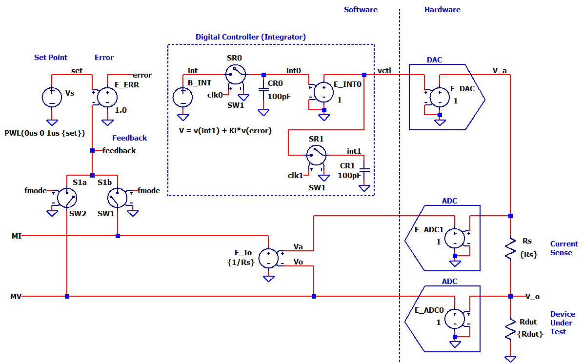
What are the basic blocks of a digital SMU? Both analog and digital SMU's carry similar functions. However, digital SMU's import many key functions into the Software. What's the advantage? Software not only reduces the amount of hardware, but offers flexibility in functions, gains and settings.

Get a review of the basic blocks.

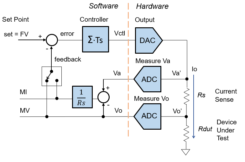
Many SMU functions have been pulled into the Software (Set Point, Error Calc, Controller). The most challenging block is the Digital Controller or Integrator (see below.)

The Hardware provides the interface to the real world through Analog / Digital Converters (DAC, ADCs). Both the DAC and ADC's have analog operating ranges of 0 to 5V.

The current sense resistor (Rs = 100ohms) consumes 0.5V max of the 5V range. This leaves 4V for the actual voltage range and the remaining 0.5V for design margin.

Lastly, the reason for the SMU is the Device Under Test (DUT), in this case a resistor Rdut.

DIGITAL CONTROLLER

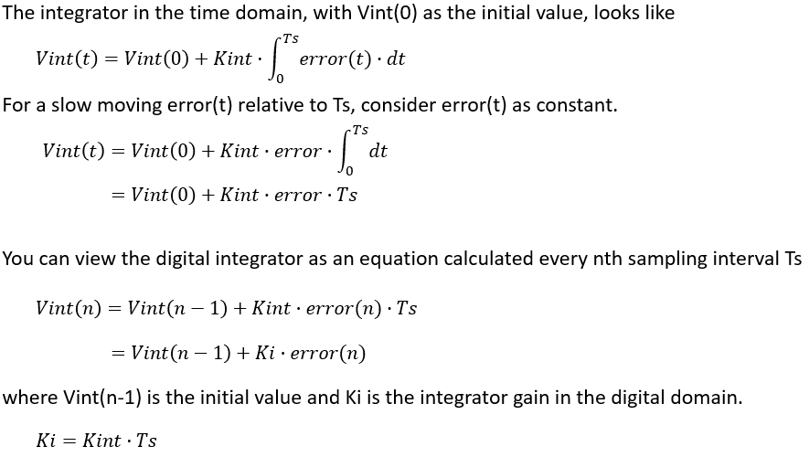
INTEGRATOR THEORY

The integrator keeps a running sum of the error signal.

For a larger error, the integrator rises more rapidly toward the desired value.
For a smaller error, the integrator moves more slowly towards the target.

What happens when the feedback reaches the set point? The error goes to zero and the integrator output holds steady.

How can we transform an analog integrator into a digital version in software? You can think of the software as calculating the integrator's output at every sampling interval Ts. A little theory can bridge the analog and digital domains.

While more complex digital models of the integrator exist, this simple version builds a basic understanding and intuition of this key block.

SPICE CIRCUIT

Here's one SPICE implementation that captures the Software's function of the digital integrator.

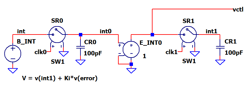
The circuit should calculate the running sum of error using current (n) and previous (n-1) values. (See section above.)

int(n) = int(n-1) + Ki * error

In SPICE, the source E_INT calculates this as

V = v(int1) + Ki * v(error)

Capacitors CR0 and CR1 act as "storage registers" for the current sum (int0) and previous sum (int1).

Switch SR0 turns on briefly in the sampling interval to capture the current sum (int0) onto CR0.
Switch SR1 turns on later in the interval to capture the value (int1) onto CR1 as the previous sum for the next calculation.

Other SPICE models are possible - some implementations use transmission line delays as storage elements.

SPICE OVERVIEW

How can we create a SPICE circuit to mimic the software functions? While just an approximation, a SPICE circuit can capture the spirit of the software functions. Many simulation possibilities exist! Here's one implementation to build some hands-on understanding and intuition.

SOFTWARE

V_SET creates a voltage for the FV or FI set level
- Force Voltage: set = FV (0 to 5V)
- Force Current: set = FI (0 to 5mA)
E_ERR calculates the error.
error = set - feedback
CONTROLLER (see discussion above)
E_MI calculates the current through the sense resistor.
MI = (Va - Vo) * 1/Rs
V_FMODE selects the feedback per fmode
- FV: fmode = 0V, S1 = ON, S2 =OFF, vfb = MV
- FI: fmode = 5V, S1 = OFF, S2 =ON, vfb = MI

ANALOG / DIGITAL INTERFACE

E_DAC provides an analog output voltage from the digital value Vctl0.
E_ADC1 converts analog voltage (Va') to a digital value (Va).
E_ADC0 converts analog voltage (Vo') to a digital value (Vo).
While very simplistic models, they allow us to focus on the control loop.

CURRENT SENSE AND DUT

Rs senses the output current.
Rdut is our Device Under Test (DUT).

EXCEL FILE

Explore the hands-on spreadsheet with the circuit calculations!

Excel file: SMU-digital-lite-1.xlsx
Right Click on filename, select "Save link as...".
Play in the sandbox, modify values, predict the impact on circuit!
Copy to a new file - experiment!

SIMULATION

Let's see the Digital SMU circuit in action. For FV or FI mode, just enable / comment the relevant .PARAM statements:

FV Mode, enable the SPICE Directive:
.param fmode=0 set=5.0V Rs=1k Rdut=20k Kint=10000

Comment out the FI params:
*.param fmode=5V ...
FI Mode, enable the SPICE Directive:
.param fmode=5V set=0.005A Rs=100 Rdut=50 Kint=20000

Comment out the FV params:
*.param fmode=0V ...

FV MODE Enable the .PARAMs for FV mode and run a TRAN simulation of SMU-FVFI-ciruit-1.cir (or *.asc). Add traces v(set) and v(feedback). Does v(feedback) rise to the set point v(set)?

Check out how the output (feedback) stair steps every Ts interval toward the desired value. Add a plot, then add traces v(error) and v(int0). Notice the operation of the digital integrator (int = int1 + Ki*error): as the error gets smaller, the increments of the running sum get smaller (int0).

Let's see how speed control works! Adjust Kint up by 2x or 3x and rerun the simulation. Does the output rise faster or slower?

FI MODE Enable the .PARAMs for FI mode and run a TRAN simulation. Does the v(feedback) rise to the desired set point v(set)?

Adjust Kint up by 2x or 3x and rerun the simulation. Does the output rise faster or slower?

SPICE NETLIST