Simplify Sensitivity Analysis

Difference vs Derivative Methods

 

Computing Sensitivities can be challenging using Derivatives. This topic walks through an example using both the Derivative Method and the quicker Difference Method using simple algebra.

Back to EBA Series

SENSITIVITY

Quick Sensitivity review:

• Sensitivity S indicates a how specific circuit characteristic will change for a given component change.
• Suppose you calculated S = 0.5 for a gain change given a resistance change.
• This means, a resistance change of 1% would cause a gain change of
   1% x 0.5 = 0.5%

 

DIFFERENCE METHOD

The Difference method calculates the sensitivity of a circuit characteristic y=f(x) over a small interval of component change Δx. From basic calculus, we get a rate of change using normalized ratios

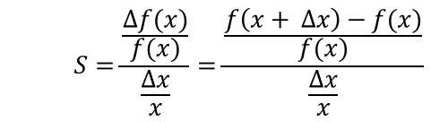
For a small Δx, the method closely estimates the actual derivative. Also note, no new function is introduced, only the original f(x).

DERIVATIVE METHOD

The Derivative Method calculates the instantaneous sensitivity of y=f(x) as the interval Δx approaches 0.

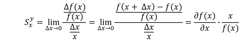
Notice, this method introduces a new function - the partial derivative. You can derive partial derivatives by applying various rules of differentiation (Chain, Product, Power, etc.).

The UPSIDE here is the potential insight gained from the new function. Not only can you develop an intuitive feel for S, but the function may also show how circuits can be optimized to minimize sensitivities. The DOWNSIDE is that deriving partial derivatives, even for simple circuits, can be a daunting and mistake prone task.

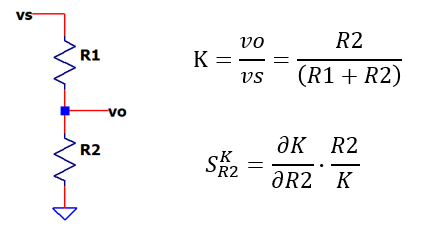
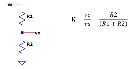
RESISTOR DIVIDER

We’ll showcase a simple, widely used resistor divider with gain K.

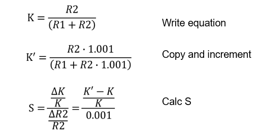
DIFFERENCE METHOD

Three steps implement the method

1. Write the original function.
2. Copy the function and increment x.
3. Calculate S

As an example, we’ll find the Sensitivity of K to R2.

For R1=750, R2=250 and an R2 increment of 0.001, we get

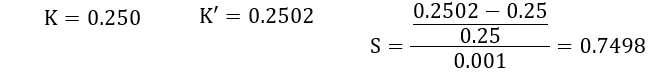
S computes fast and easy. However, no further insight is provided.

 

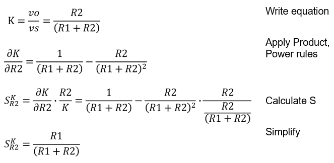
DERIVATIVE METHOD

Let’s see the Derivative Method in action.

1. Write the original function
2. Derive partial derivative function using rules: Chain, Product, Powers, etc.
3. Calculate S and simplify
   

For R1=750, R2=250, we get

  S = 0.750

Good news, the Derivative method confirms the Difference method’s result S = 0.7498. (An increment of 0.0001 or less, gets you even closer.)

As you can see, the Derivative method requires more mathematical effort then the Difference Method. However, the equation reveals how S scales relatively with the signal lost across R1 - more or less attenuation means more or less sensitivity, respectively!

I also found S satisfying and fun to derive using my calculus skills that admittedly needed a refresh cycle. Unfortunately, when analyzing a large number of more complex circuits, the sensitivities could quickly become tedious and error prone.

TRY IT!

What is the Sensitivity for an R Divider with R1=1k and R2=1k?

 

Back to EBA Series